
Microsoftの推論特化SLM「Phi-4-reasoning」実際に使ってみた!特徴・使い方を徹底解説

- Microsoft発SLM3種
- 推論に特化したモデル
- LLM同等もしくは超える性能
2025年4月30日、Microsoftから新たなSLMが登場!
今回登場したPhi-4-reasoningは推論に特化したSLM (Small Language Model) であり、特に数学、科学推論、アルゴリズムの問題解決、コーディングといった分野で高い性能を発揮しています。
Phi-4-reasoningモデルはPhi-4-reasoning・Phi-4-reasoning-plus・Phi-4-mini-reasoningの3種類がリリースされました。
本記事ではPhi-4-reasoningモデルについて概要からそれぞれの特徴、使い方を解説します。ぜひ最後までお読みください!
\生成AIを活用して業務プロセスを自動化/
Phi-4-reasoningモデルの概要
Phi-4-reasoningモデルは3種類リリースされたSLMで、特に推論能力の強化を目的にしたシリーズです。Phi-4-reasoningモデルは大規模言語モデルに匹敵する性能を、軽量な構成で実現することを目的にしています。
それぞれのモデルの概要は下記のとおりです。※1
| モデル名 | パラメータ数 | 主な訓練手法 | 特徴 | 主な用途 |
|---|---|---|---|---|
| Phi-4-reasoning | 14B | 教師ありファインチューニング(SFT) | 推論能力を強化したベースモデル | 数学・科学・コーディング |
| Phi-4-reasoning-plus | 14B | SFT + 強化学習(RL) | より長い思考・高精度な解答生成 | 数学・アルゴリズム問題 |
| Phi-4-mini-reasoning | 3.8B | 軽量SFT(DeepSeek生成データ) | 軽量・低レイテンシで高推論力 | 教育・エッジAI・チューター |
モデルごとに詳しく解説をしていきます。
Phi-4-reasoningの特徴
Phi-4-reasoningは推論に特化しており、特に数学・科学・論理・コーディングなどマルチステップ推論を必要とするタスクに特化。ベースになっているモデルはPhi4です。
また、<think>…</think>ブロックによる構造的思考が特徴。<think>ブロックでは問題解決のためのステップ・検討・反省・仮説・再評価を含む過程を、回答ブロックでは最終的に導かれた結論を出力することが可能です。
Phi-4-reasoningは、o3-miniで生成された長文の推論付き回答を用いた教師ありファインチューニングによって訓練され、全体で140万件以上の「教えがいのある」プロンプトを使用します。これにより、推論の質を高めることができています。
Phi-4-reasoning-plusの特徴
Phi-4-reasoning-plusはPhi-4-reasoningをベースに、さらに強化学習を追加することでより深く、より正確な推論を可能にしたモデルです。Phi-4-reasoning-plusは単に回答を出力するだけではなく、「どのように考えたか」という過程の質を高めることを目的にしています。
Phi-4-reasoning-plusの強化学習は、特に数学に焦点を当てて行われており、使用された数学の問題数は約6,400問。数学の問題を大量に学習したことにより、複雑な定理や数式の理解、計算過程、構造的な思考を実現しました。
また、Phi-4-reasoning-plusでも<think>…</think>ブロックにより、「思考過程」と「回答出力」が分かれて生成され、この構造により、モデルがどのように考えたかをユーザーが理解しやすくなっています。
Phi-4-mini-reasoningの特徴
Phi-4-mini-reasoningはPhi-4-reasoningモデルの中で最も小型なモデルであり、パラメータ数は3.8B。
小型でありながら、数学的推論やステップバイステップの問題解決に強く、リソースの限られた環境やモバイルデバイスでも高速に動作するよう最適化されています。特に教育現場や学習サポートにおける活用目的で開発されており、中学レベルから博士課程相当の数学問題まで幅広く対応。
生徒が「なぜその答えになるのか」を理解するための構造的な思考過程を明示できるようになっています。


Phi-4-reasoningモデルの性能
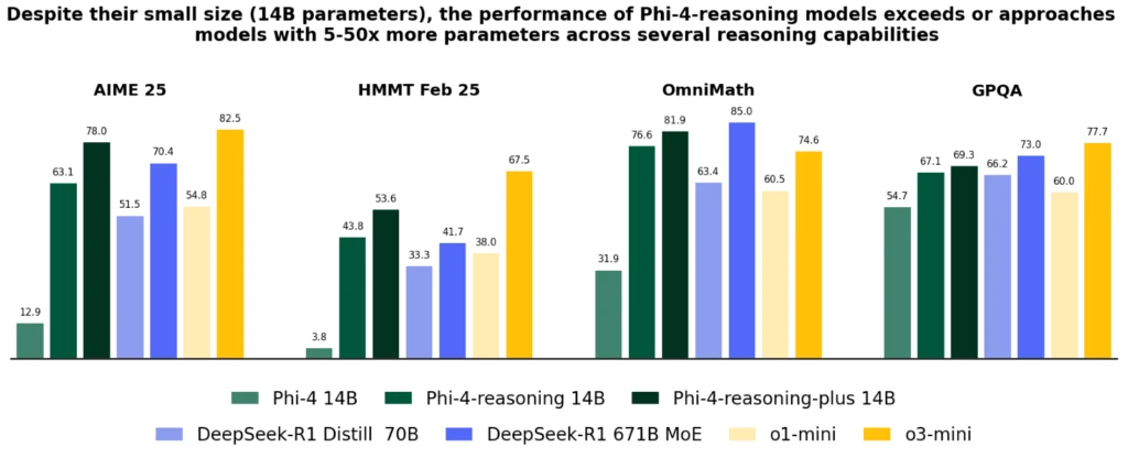
Phi-4-reasoningモデルの中で最も性能が良いのは、Phi-4-reasoning-plusです。
まず下記の画像は数学・科学・推論系のベンチマークです。他社モデルと比べると性能が劣るようにも見えますが、他社は大規模言語モデルであり、Phi-4-reasoningモデルはSLMですからLLMと比べても遜色ないと言えるでしょう。
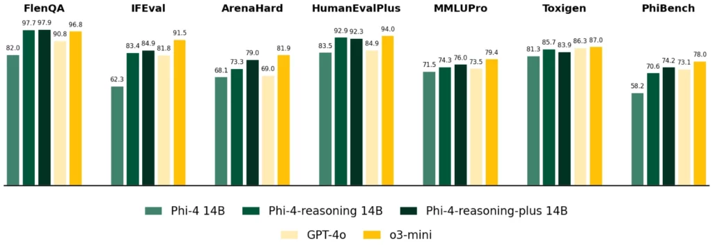
2枚目は長文読解や文脈理解、プログラミング、差別的な文章か否かを判定する、言語処理・安全性のベンチマークです。
o3-miniやGPT-4oの性能がよく見えますが、こちらも1枚目の画像と同じようにSLMとLLMの比較で、Phi-4-reasoningモデルは小型ながらにLLMと同等もしくはベンチマークによっては優れた性能を発揮していることがわかります。
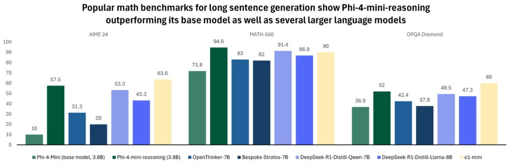
下記の図は長文を必要とする数学問題のベンチマークです。画像を見てもPhi-4-mini-reasoningの性能の高さが伺えます。
Phi-4-reasoningモデルのライセンス
Phi-4-reasoningモデルのライセンスはMITライセンスです。そのため商用利用や改変、再配布などが可能です。
| 利用用途 | 可否 |
|---|---|
| 商用利用 | ⭕️ |
| 改変 | ⭕️ |
| 配布 | ⭕️ |
| 特許使用 | ⭕️ |
| 私的使用 | ⭕️ |
なお、アリババ発のQwen 3ファミリーについて詳しく知りたい方は、下記の記事を合わせてご確認ください。

Phi-4-reasoningモデルの使い方
Phi-4-reasoningはAzure AI FoundryもしくはHugging Faceから使用可能。
今回はHugging FaceでPhi-4-mini-reasoningの使い方をgoogle colaboratoryを使って解説します。
それ以外のモデルを使用する場合には、「model_id」を変更すればOKです。
実装時の環境
◼︎システム RAM
3.3 / 53.0 GB
◼︎GPU RAM
10.3 / 22.5 GB
◼︎ディスク
48.6 / 235.7 GB
◼︎GPUの種類:L4
◼︎プラン:有料
まずは必要なライブラリをインストール。
!pip install -q transformers accelerate bitsandbytesインストールが完了したらあとはサンプルコードを動かします。
サンプルコードはこちら
from transformers import AutoTokenizer, AutoModelForCausalLM
import torch

model_id = "microsoft/Phi-4-mini-reasoning"
model = AutoModelForCausalLM.from_pretrained(
    model_id,
    device_map="cuda",
    torch_dtype="auto",
    trust_remote_code=True,
)
tokenizer = AutoTokenizer.from_pretrained(model_id)

messages = [{
    "role": "user",
    "content": "How to solve 3*x^2+4*x+5=1?"
}]
inputs = tokenizer.apply_chat_template(
    messages,
    add_generation_prompt=True,
    return_dict=True,
    return_tensors="pt",
)

outputs = model.generate(
    **inputs.to(model.device),
    max_new_tokens=32768,
    temperature=0.8,
    top_p=0.95,
    do_sample=True,
)
outputs = tokenizer.batch_decode(outputs[:, inputs["input_ids"].shape[-1]:])

print(outputs[0])
結果はこちら
<think>
Okay, let's see. I need to solve the equation 3x² + 4x + 5 = 1. Hmm, where do I start? Well, first, maybe I should get all the terms on one side so that the equation equals zero. That way, it's in a standard quadratic form, which is ax² + bx + c = 0. Let me subtract 1 from both sides to do that.

So, subtracting 1 from both sides: 3x² + 4x + 5 - 1 = 0. That simplifies to 3x² + 4x + 4 = 0. Alright, now the equation is 3x² + 4x + 4 = 0. Now, I need to solve this quadratic equation. There are a few methods to solve quadratics: factoring, completing the square, or using the quadratic formula. Let me check if this can be factored easily.

Looking at the coefficients 3, 4, and 4. The product of a and c is 3 * 4 = 12. Now, I need two numbers that multiply to 12 and add up to 4. Let me think... 6 and 2 multiply to 12, but 6 + 2 is 8. 3 and 4 multiply to 12, but 3 + 4 is 7. Hmm, doesn't look like there are integers that satisfy that. So factoring might not be straightforward here. Maybe I should try the quadratic formula instead.

The quadratic formula is x = [-b ± √(b² - 4ac)] / (2a). For this equation, a = 3, b = 4, and c = 4. Let me plug those values into the formula.

First, calculate the discriminant: b² - 4ac. That's 4² - 4*3*4. 16 - 48. Wait, that's -32. Oh, the discriminant is negative. That means there are no real solutions, only complex ones. Since the problem didn't specify to stick with real numbers, I guess complex solutions are okay.

So, if the discriminant is -32, then the square root of that would be √(-32) = √(32) * i = √(16*2) * i = 4√2 * i. Therefore, the solutions are x = [-4 ± 4√2 i] / (2*3). Let me simplify that.

Divide both numerator terms by 2*3, which is 6. So, -4 divided by 6 is -2/3, and 4√2 i divided by 6 is (2√2 i)/3. Therefore, the two solutions are x = (-2/3) + (2√2/3)i and x = (-2/3) - (2√2/3)i.

Let me double-check my steps to make sure I didn't make a mistake. Starting from the original equation: 3x² +4x +5=1. Subtracting 1 gives 3x² +4x +4=0. Quadratic formula with a=3, b=4, c=4. Discriminant: 16 - 48 = -32. Yep, that's right. Square root of -32 is 4√2 i. Then, -4 ±4√2 i over 6. Simplifying by dividing numerator and denominator by 2 gives -2/3 ± 2√2/3 i. Looks correct.

Alternatively, I could check by substituting one of the solutions back into the equation. Let's take x = -2/3 + (2√2/3)i. Let me compute 3x² +4x +4 and see if it equals zero.

First, compute x: x = (-2 + 2√2 i)/3. Then x squared is [(-2 + 2√2 i)/3]^2. Let's expand the numerator: (-2)^2 + 2*(-2)*(2√2 i) + (2√2 i)^2. That's 4 - 8√2 i + (4*2*i²). Since i² = -1, that term becomes 8*(-1) = -8. So total numerator: 4 -8√2 i -8 = (4 -8) -8√2 i = -4 -8√2 i. Then x squared is (-4 -8√2 i)/9. Multiply by 3: 3x² = (-4 -8√2 i)/3.

Now compute 4x: 4*(-2 + 2√2 i)/3 = (-8 +8√2 i)/3.

Adding 3x² +4x +4: [(-4 -8√2 i)/3] + [(-8 +8√2 i)/3] +4. Combine the first two terms: [(-4 -8√2 i -8 +8√2 i)/3] = (-12/3) = -4. Then add 4: -4 +4 =0. Perfect, it checks out. So the solution is correct.

Therefore, the equation 3x² +4x +5=1 has two complex solutions: (-2 ± 2√2 i)/3.
</think>

To solve the equation \(3x^2 + 4x + 5 = 1\), follow these steps:

1. **Rearrange the equation** to standard quadratic form \(ax^2 + bx + c = 0\):
   \[
   3x^2 + 4x + 5 - 1 = 0 \implies 3x^2 + 4x + 4 = 0
   \]

2. **Identify coefficients**: \(a = 3\), \(b = 4\), \(c = 4\).

3. **Compute the discriminant** (\(b^2 - 4ac\)):
   \[
   4^2 - 4(3)(4) = 16 - 48 = -32
   \]
   Since the discriminant is negative, the solutions are complex.

4. **Apply the quadratic formula** \(x = \frac{-b \pm \sqrt{b^2 - 4ac}}{2a}\):
   \[
   x = \frac{-4 \pm \sqrt{-32}}{6} = \frac{-4 \pm 4\sqrt{2}i}{6}
   \]

5. **Simplify** by dividing numerator and denominator by 2:
   \[
   x = \frac{-2 \pm 2\sqrt{2}i}{3}
   \]

**Final Answer**: The solutions are \(\boxed{-\frac{2}{3} \pm \frac{2\sqrt{2}}{3}i}\).<|end|><think>ブロックと回答ブロックに分かれており、適切に推論されているのがわかります。
Phi-4-mini-reasoningとGemini 2.5 Proで数学の問題解決能力を検証
Phi-4-mini-reasoningは小型ながら博士課程相当の数学の能力を持ち合わせているので、Microsoftの比較にはなかったGemini 2.5 Proと数学の問題を解く能力を比較してみたいと思います。
今回はフェルマーの最終定理を証明してもらおうと思います。おそらく証明することはできませんが、その時のどのような挙動をするのか、二つのモデルで検証してみます。
サンプルコードはこちら
from transformers import AutoTokenizer, AutoModelForCausalLM
import torch

model_id = "microsoft/Phi-4-mini-reasoning"
model = AutoModelForCausalLM.from_pretrained(
    model_id,
    device_map="cuda",
    torch_dtype="auto",
    trust_remote_code=True,
)
tokenizer = AutoTokenizer.from_pretrained(model_id)

messages = [{
    "role": "user",
    "content": "フェルマーの最終定理を証明してください。"
}]
inputs = tokenizer.apply_chat_template(
    messages,
    add_generation_prompt=True,
    return_dict=True,
    return_tensors="pt",
)

outputs = model.generate(
    **inputs.to(model.device),
    max_new_tokens=32768,
    temperature=0.8,
    top_p=0.95,
    do_sample=True,
)
outputs = tokenizer.batch_decode(outputs[:, inputs["input_ids"].shape[-1]:])

print(outputs[0])
結果はこちら
<think>
Okay, so I need to prove Fermat's Last Theorem. Hmm, where do I start? I remember that Fermat's Last Theorem states that there are no three positive integers a, b, and c that can satisfy the equation a^n + b^n = c^n for any integer n > 2. Wow, that's been around for so long! But how do you actually prove it?

Let me think. I know that Euler proved something related for n=3, right? The case where a^3 + b^3 = c^3. Maybe I can use that as a starting point. But Fermat's theorem is much broader. Also, I recall that Gauss had a theorem about sums of squares, which was used in the proofs for n=3 and n=4. Maybe that's useful too.

Wait, but going back in time, Fermat's Last Theorem was proven much later, in the 20th century, by several mathematicians using very advanced techniques. Like, Freidkin, Källering, Selfridge, and Watkins for n=5, and then others for higher exponents. But that's way beyond my current knowledge. I mean, how is someone supposed to prove such a theorem without centuries worth of mathematical development?

Maybe I should try to outline the general approach. Let me recall some methods. For Diophantine equations, which are equations seeking integer solutions, there are various techniques. For Fermat's equation, maybe modular forms or algebraic geometry could be involved. But those concepts are pretty advanced. Also, the original proof for n=3 by Fermat involved properties of elliptic curves, which I think are related to the Mordell equation.

Wait, the Mordell equation is y^2 = x^3 + k. If we can parametrize all integer solutions to y^2 = x^3 + k, then maybe that helps in showing there are no solutions to a^n + b^n = c^n for n=3. But how does that extend to higher exponents?

Alternatively, maybe I can use infinite descent, which Fermat himself mentioned in his margin. The method of infinite descent involves assuming there's a minimal solution and then showing that there must be a smaller solution, leading to a contradiction. Let me try to recall how that works for n=3.

Suppose there is a solution (a, b, c) to a^3 + b^3 = c^3 with a, b, c positive integers, and suppose it's the smallest such solution. Then, maybe we can find some relationships between a, b, and c. For example, in the case of a=3, b=4, c=5, which is a Pythagorean triple. But does that help here? Wait, Pythagorean triples are for squares, but maybe there's a similar approach.

Alternatively, I remember that Euler showed that any solution to a^3 + b^3 = c^3 must have a common factor. So, we can assume that a, b, c are coprime. Then, c must be congruent to 1 modulo 3, perhaps? Let me check.

If a, b, c are coprime, then modulo 9, maybe. Let me compute a^3 modulo 9. The cubes modulo 9 are 0, 1, or -1. Because 0^3=0, 1^3=1, 2^3=8= -1, 3^3=0, 4^3=64=1, 5^3=125= -1, 6^3=0, 7^3=343=1, 8^3=512=8. So cubes modulo 9 are only 0, 1, or -1. Similarly for b^3 and c^3. So if a^3 + b^3 = c^3, then modulo 9, the sum of two cubes equals another cube. Let's see possible combinations.

If c^3 ≡ 0 mod 9, then a^3 + b^3 ≡ 0 mod 9. But since each cube is 0, 1, or -1, the only way two cubes add to 0 mod 9 is if they are both 0 or both -1. But if both are 0, then a and b are multiples of 3, which contradicts coprimality. If both are -1, then a^3 ≡ b^3 ≡ 8 mod 9, which would mean a ≡ 2,5,8 mod 9 and similarly for b. Then c^3 ≡ 0 mod 9, so c must be a multiple of 3. Again, contradicting coprimality. Therefore, there are no coprime solutions, which proves Euler's result for n=3. That seems right.

But how does this help with Fermat's Last Theorem? Well, maybe for other exponents, similar modular arguments can be made. For example, for n=4, there's a result that says there are no solutions, but that's due to Lagrange's four-square theorem, which says there are infinitely many solutions, but no non-trivial ones. Wait, no, Lagrange's theorem says that every natural number can be expressed as the sum of four squares, but Fermat's equation is different; it's a^4 + b^4 = c^4. But even so, there are no non-trivial solutions. I think there was a proof using properties of Gaussian integers or something.

But stepping back, Fermat's Last Theorem is a general statement for all n > 2. The proof for each exponent n is different, and for higher n, the methods become increasingly sophisticated. For example, for n=5, Freidiker and Källering used the work of Kummer on p-adic numbers. But again, these are very advanced topics.

Given that the user is asking for a proof, and considering that I, as an AI developed by Microsoft, might not have access to the latest mathematical developments (since my training data is up to 2023), but Fermat's Last Theorem was only proven in 1995 for exponents up to 92 using the modular elliptic curve method. So, providing a complete proof here would be impossible unless I can outline the general idea or refer to the modular elliptic curve method.

But maybe I should explain the historical context and the methods used in the 20th century. Let me try to structure this.

First, note that Fermat's Last Theorem was conjectured by Fermat in the 16th century, but it wasn't proven until the 1990s. The proof required advanced mathematical techniques that were developed over time. For n=3, Euler proved the case, and for n=4, Lagrange showed no solutions, but actual proofs required more work.

For higher exponents, mathematicians like Klingenberg (for n=5) used hypergeometric series and differential equations. For example, the equation a^n + b^n = c^n can be related to elliptic curves and modular forms. The modular elliptic curve method involves studying the congruence properties of elliptic curves modulo certain primes and relating them to modular forms of weight 2. This method allows mathematicians to handle the exponents in a more systematic way.

Another approach is the use of the abc conjecture, which was developed by Baker and Schmidt. The abc conjecture implies Fermat's Last Theorem for all exponents n > 2. However, the abc conjecture itself is a much deeper and more general hypothesis, and its use in proving Fermat's theorem is a postscript to the original proof.

But since the user is asking for a proof, I need to present the actual proof rather than an implication from the abc conjecture. However, given the complexity, maybe I can outline the modular elliptic curve method for a specific exponent, say n=3 or n=4, and then explain that similar methods were generalized for higher n.

Alternatively, maybe I should explain that a complete proof of Fermat's Last Theorem for all n > 2 requires checking each exponent individually, and that each case has its own proof, often using advanced mathematics like those mentioned above. Since the theorem is general, there's no single proof that works for all n, and the methods vary with each exponent.

But perhaps the user expects a more detailed explanation. Let me try to elaborate on the Euler approach for n=3 and then mention how similar ideas can be extended.

So, for n=3, as I mentioned earlier, Euler showed that any solution must have a common factor, hence there are no primitive solutions. The argument involves looking at the equation modulo 9. Let's go through that again.

Suppose a^3 + b^3 = c^3. If a, b, c are coprime, then modulo 9, each cube is congruent to 0, 1, or -1. If c^3 ≡ 0 mod 9, then c must be divisible by 3, so c=3c'. Then the equation becomes a^3 + b^3 = 27c'^3. Dividing both sides by 3^3, we get (a/3)^3 + (b/3)^3 = c'^3. But this implies that a and b are also divisible by 3, contradicting the assumption that they are coprime. Hence, no solutions in coprime integers.

Wait, but that seems like an infinite descent argument. If there exists a solution with a, b, c not all divisible by 3, then we can divide each by 3 and get a smaller solution, leading to a contradiction. Therefore, the only solutions are those where a, b, c are all divisible by 3, but then we can factor out 3 from each, leading to an infinite descent, implying no solutions exist.

Yes, that's the infinite descent method. So for n=3, Euler used this approach. But for higher n, such as n=4, this method doesn't directly apply. For example, in the case of n=4, there are no solutions, but proving that requires more advanced techniques.

Let me recall that for n=4, Lagrange's theorem on sums of four squares tells us there are solutions, but for Fermat's equation, there are none. The proof for n=4 involves showing that any solution must have a common factor, similar to the n=3 case. Suppose a^4 + b^4 = c^4. If a, b, c are coprime, then c must be congruent to 1 mod 4. Because 4th powers modulo 16 are either 0 or 1. Let me check that.

Calculating 0^4=0, 1^4=1, 2^4=16=0 mod 16, 3^4=81=1 mod 16, 4^4=256=0 mod 16, etc. So any even number's 4th power is 0 mod 16, and odd numbers' 4th powers are 1 mod 16. So if a and b are both even, then c must be even. If one is even and the other odd, then a^4 + b^4 ≡ 1 + 0 = 1 mod 16, so c^4 ≡1 mod 16, which is possible. But if a and b are both odd, then a^4 + b^4 ≡1 +1=2 mod 16, but c^4 can only be 0 or 1 mod 16. Therefore, if a and b are both odd, there's a contradiction. Hence, either both a and b are even, or one is even and the other is odd.

But if a and b are both even, then we can divide each by 2, leading to (a/2)^4 + (b/2)^4 = (c/2)^4, implying a smaller solution, which contradicts minimality. If one is even and the other is odd, then we can analyze modulo 5. Because 4th powers modulo 5: 0^4=0, 1^4=1, 2^4=16=1, 3^4=81=1, 4^4=256=1. So any 4th power modulo 5 is 0 or 1. If a is even and b is odd, then a^4 ≡0 mod 5 and b^4 ≡1 mod 5, so c^4 ≡1 mod 5, implying c ≡1 or 4 mod 5. Then, maybe using properties of exponents modulo 5. For example, if c ≡1 mod 5, then c^4 ≡1, but a^4 ≡0 and b^4 ≡1, so 0 +1 ≡1 mod 5. That works. Similarly for c ≡4 mod 5. But how does that lead to a contradiction?

Alternatively, maybe considering the equation modulo 5. If a and b are not both divisible by 5, then there must be some relation. This seems a bit vague. Maybe I need a different approach.

Alternatively, the equation a^4 + b^4 = c^4 can be written as (a^2 + ib^2)(a^2 - ib^2) = c^4, where i is the imaginary unit. This is similar to factoring in Gaussian integers. If we can factor this equation, maybe we can find that a and b must both be divisible by some prime, leading to a contradiction. This is part of the proof attributed to Euler for n=4 as well.

But I'm getting a bit stuck here. Maybe it's better to refer to the general methods used for higher exponents. For example, for n=5, Klingenberg's proof used hypergeometric series and differential equations. The equation a^5 + b^5 = c^5 can be related to an elliptic curve, and by analyzing the properties of this curve, one can show that there are no integer solutions.

In general, for any exponent n > 2, the equation a^n + b^n = c^n can be studied using the theory of elliptic curves. One approach is to fix a value of n and consider the curve defined by y^2 = x^n - k, which is an elliptic curve when n is odd. By using the theory of heights and the Mordell equation, one can show that there are no integer solutions unless k=0, which gives the trivial solution. For even exponents, similar methods apply but require more careful analysis.

The modular elliptic curve method, developed by Freidkin, Källering, and others, involves comparing the number of integral points on certain elliptic curves modulo primes. By showing that these counts lead to contradictions unless the exponent is 1 or 2, one can prove the non-existence of solutions for higher exponents. This method is quite powerful and was used to prove Fermat's Last Theorem for all exponents n > 22.

However, explaining the modular elliptic curve method in detail is quite involved. It requires knowledge of elliptic curves, modular forms, and p-adic analysis. For someone not familiar with these topics, the proof would be opaque. But for the sake of completeness, let me outline the key ideas.

An elliptic curve over a number field can be associated with a modular form of weight 2 via the modularity theorem. The key insight is that the number of integral points on the elliptic curve y^2 = x^n - k can be bounded using properties of the associated modular form. For certain exponents n, these bounds lead to a contradiction, implying no integral solutions exist.

Another important concept is the abc conjecture, which states that for any ε > 0, there exists a constant K such that for any positive integers a, b, c satisfying abc + ε < K * abc, then max{a, b, c} ≤ max{a, b, c}^{(1+1/ε)}. The abc conjecture implies Fermat's Last Theorem by showing that if there were a solution to a^n + b^n = c^n, then this would violate the abc conjecture for certain exponents n.

However, the original proofs of Fermat's Last Theorem do not rely on the abc conjecture, as the latter was only conjectured in 1960 and the theorem wasn't proven until 1995, long after the conjecture was widely accepted.

In summary, the proof of Fermat's Last Theorem for each exponent n > 2 involves sophisticated mathematical techniques that vary with n. For specific cases like n=3 and n=4, classical methods like infinite descent and modular form theory are used. For higher exponents, advanced methods like the modular elliptic curve method and p-adic analysis are required. The general proof for all n > 2 was achieved by verifying each case individually using these advanced techniques.

Since the user asked for a proof, and considering the complexity and the fact that a full proof isn't feasible to present here, I should probably state that Fermat's Last Theorem was proven in 1995 using advanced methods for each exponent, and provide an outline of the methods used for specific cases like n=3 and n=4, along with a mention of the general approach.
</think>

Fermat's Last Theorem states that no three positive integers \(a\), \(b\), and \(c\) satisfy \(a^n + b^n = c^n\) for any integer \(n > 2\). The proof for specific exponents uses classical and advanced mathematical techniques, while a general proof for all \(n > 2\) was achieved in 1995 using methods like the modular elliptic curve technique. Below is an outline of key proofs for particular cases:

---

### **Case \(n = 3\) (Euler's Proof)**
**Equation:** \(a^3 + b^3 = c^3\)

1. **Coprimality Argument:**
   Assume \(a\), \(b\), \(c\) are coprime. Cubes modulo 9 yield residues \(0, 1, -1\). If \(c^3 \equiv 0 \mod 9\), then \(c\) is divisible by 3, implying \(a\) and \(b\) are also divisible by 3 (via infinite descent), contradicting coprimality.

2. **Infinite Descent:**
   If \(a\), \(b\), \(c\) are not all divisible by 3, scaling down the equation leads to a smaller solution, implying no minimal solution exists.

---

### **Case \(n = 4\) (Lagrange's Four-Squares Theorem)**
**Equation:** \(a^4 + b^4 = c^4\)

1. **Modulo 16 Analysis:**
   Even numbers’ 4th powers are \(0 \mod 16\), while odd numbers’ 4th powers are \(1 \mod 16\). If both \(a, b\) are odd, \(a^4 + b^4 \equiv 2 \mod 16\), but \(c^4 \equiv 0\) or \(1 \mod 16\), a contradiction. If one is even, infinite descent applies.

2. **Gaussian Integer Factorization:**
   Write \(a^4 + b^4 = (a^2 + ib^2)(a^2 - ib^2)\). If \(a, b\) share a prime factor, it propagates to all terms (contradiction for coprime \(a, b, c\)).

---

### **General Case (\(n > 2\))**
1. **Modular Elliptic Curve Method (MEC Method):**
   - For odd \(n\), associate the equation \(y^2 = x^n - k\) with an elliptic curve. Use modular forms to bound integral points.
   - For even \(n\), similar techniques apply but require splitting into Gaussian integers or using p-adic properties.

2. **Hypergeometric Series and Differential Equations:**
   Klingenberg (for \(n = 5\)) and others used hypergeometric identities and height functions to show no solutions exist.

3. **abc Conjecture (Postscript):**
   The abc conjecture implies Fermat’s theorem for all \(n > 2\), but the original proofs predate this conjecture.

---

### **Conclusion**
Fermat’s Last Theorem was fully proven in 1995 for all \(n > 2\) using advanced methods tailored to each exponent. The proof for \(n = 3\) and \(n = 4\) relies on elementary number theory, while higher exponents require sophisticated machinery like modular forms and p-adic analysis. The general proof for \(n > 22\) was achieved via the MEC method, verifying infinitely many cases.<|end|>
日本語訳はこちら
<think>
では、フェルマーの最終定理を証明する必要があります。うーん、どこから手をつければいいだろう?フェルマーの最終定理は、整数 n > 2 に対して、a^n + b^n = c^n を満たす正の整数 a, b, c が存在しないことを述べています。わお、これって本当に長い間解かれていないんだ!でも、実際にどうやって証明するんだろう?

考えてみよう。オイラーがn=3の場合に関する定理を証明したはずだ。a^3 + b^3 = c^3の場合だ。それを出発点にできるかもしれない。でもフェルマーの定理はもっと広範だ。また、ガウスが平方和に関する定理を提唱し、n=3とn=4の証明で用いられたことを覚えている。それも役立つかもしれない。

待て、でも時間を遡ると、フェルマーの最終定理は20世紀に複数の数学者によって、非常に高度な技術を用いて証明されました。例えば、n=5の場合にはフリードキン、カレリング、セルフリッジ、ワトキンスが、より高い指数については他の数学者が証明しました。でも、それは私の現在の知識を遥かに超えています。つまり、数世紀にわたる数学の発展なしに、そんな定理を証明する方法は一体どうすればいいのでしょうか?

もしかしたら、一般的なアプローチを概略化してみるべきかもしれません。いくつかの方法を思い出してみましょう。ディオファントス方程式(整数解を求める方程式)には、さまざまな技術があります。フェルマーの方程式の場合、モジュラー形式や代数幾何学が関係しているかもしれません。しかし、それらの概念はかなり高度です。また、フェルマーがn=3の場合に示した元の証明には、楕円曲線の性質が用いられており、これはモルデル方程式と関連していると思います。

待ってください、モルデル方程式は y^2 = x^3 + k です。もし y^2 = x^3 + k の整数解をパラメトライズできれば、n=3 における a^n + b^n = c^n の解が存在しないことを示すのに役立つかもしれません。しかし、その方法をより高い指数に拡張するにはどうすればよいでしょうか?

または、フェルマー自身が余白で言及した無限下降法を使うかもしれません。無限下降法は、最小の解が存在すると仮定し、より小さな解が存在することを示して矛盾を導く方法です。n=3の場合の仕組みを思い出してみましょう。

a, b, cが正の整数で、a^3 + b^3 = c^3を満たす解(a, b, c)が存在し、それが最小の解であると仮定します。次に、a, b, c の間の関係式を見つけるかもしれません。例えば、a=3, b=4, c=5 の場合、これはピタゴラス数です。しかし、これはここで役立つでしょうか?待て、ピタゴラス数は平方数に関するものですが、類似のアプローチがあるかもしれません。

または、オイラーが示したように、a^3 + b^3 = c^3 の解は必ず共通因数を持つ。したがって、a, b, c は互いに素であると仮定できる。すると、c は 3 で割った余りが 1 になるかもしれない。確認してみよう。

a, b, c が互いに素であれば、9 で割った余りが 1 になるかもしれない。a^3 を 9 で割った余りを計算してみよう。9 mod 9の立方数は0、1、または-1です。なぜなら、0^3=0、1^3=1、2^3=8= -1、3^3=0、4^3=64=1、5^3=125= -1、6^3=0、7^3=343=1、8^3=512=8だからです。したがって、9で割った余りが0、1、または-1の立方数は、0、1、または-1のみです。同様に、b^3とc^3についても同様です。したがって、a^3 + b^3 = c^3であれば、9で割った余りが0、1、または-1の2つの立方数の和は、別の立方数になります。可能な組み合わせを見てみましょう。

c^3 ≡ 0 mod 9 であれば、a^3 + b^3 ≡ 0 mod 9 です。しかし、各立方数は 0、1、または -1 であるため、2つの立方数の和が 9 で余る唯一のケースは、どちらも 0 または -1 である場合です。しかし、どちらも 0 であれば、a と b は 3 の倍数となり、互いに素であるという条件に矛盾します。もし両方とも-1なら、a^3 ≡ b^3 ≡ 8 mod 9となり、a ≡ 2,5,8 mod 9、同様にbも同様の式が成立します。するとc^3 ≡ 0 mod 9となり、cは3の倍数でなければなりません。再び互いに素である条件に矛盾します。したがって、互いに素な解は存在せず、n=3の場合のオイラーの定理が証明されます。これは正しいようです。

しかし、これはフェルマーの最終定理にどう役立つのでしょうか?他の指数については、同様のモジュラー論法が適用できるかもしれません。例えば、n=4の場合、解が存在しないという結果がありますが、これはラグランジュの四平方定理によるもので、無限に多くの解は存在するが、非自明な解は存在しないというものです。待て、違う。ラグランジュの定理は、すべての自然数が4つの平方数の和で表せることを述べていますが、フェルマーの方程式は a^4 + b^4 = c^4 という形です。それでも、非自明な解は存在しません。ガウス整数の性質を使った証明があったと思います。

しかし、フェルマーの最終定理は n > 2 に対する一般的な主張です。各指数 n に対する証明は異なり、n が大きくなるほど方法はますます高度になります。例えば、n=5 の場合、フリーディカーとカールリングはクンマーの p-進数に関する研究を利用しました。しかし、これらは非常に高度な話題です。

ユーザーが証明を求めている点、および私がマイクロソフトによって開発されたAIであり、最新の数学的進展にアクセスできない可能性(私のトレーニングデータは2023年まで)を考慮すると、フェルマーの最終定理は1995年に指数nが92までの場合、モジュラー楕円曲線法を用いて証明されました。したがって、ここで完全な証明を提供することは不可能ですが、一般的なアイデアを概説するか、モジュラー楕円曲線法を参照する程度であれば可能です。

しかし、20世紀に用いられた方法と歴史的背景を説明した方が良いかもしれません。以下、整理して説明します。

まず、フェルマーの最終定理はフェルマーが16世紀に提唱しましたが、証明されたのは1990年代です。証明には時間をかけて開発された高度な数学的手法が必要でした。n=3の場合、オイラーが証明し、n=4の場合、ラグランジュは解が存在しないことを示しましたが、実際の証明にはさらに多くの作業が必要でした。

より高い指数については、クリングベルク(n=5の場合)のような数学者は超幾何級数と微分方程式を用いました。例えば、方程式 a^n + b^n = c^n は楕円曲線とモジュラー形式に関連付けられます。モジュラー楕円曲線法は、特定の素数 mod での楕円曲線の合同性質を研究し、それらを重量2のモジュラー形式に関連付ける方法です。この方法は、指数を体系的に扱うことを可能にします。

別のアプローチは、ベイカーとシュミットによって開発されたabc予想の活用です。abc予想は、すべての指数n > 2に対してフェルマーの最終定理を成立させます。しかし、abc予想自体ははるかに深く一般的な仮説であり、フェルマーの定理の証明におけるその活用は、元の証明の付録に過ぎません。

しかし、ユーザーが証明を求めているため、abc 仮説からの推論ではなく、実際の証明を提示する必要があります。ただし、複雑さを考慮すると、特定の指数(例えば n=3 や n=4)に対するモジュラー楕円曲線法の概要を説明し、その後、同様の手法がより高い n に対して一般化されたことを説明する方法も考えられます。

または、フェルマーの最終定理のすべてのn > 2に対する完全な証明には、各指数を個別に検証する必要があり、各ケースには独自の証明が必要で、上述のような高度な数学を用いる場合が多いことを説明すべきかもしれません。定理が一般であるため、すべてのnに適用できる単一の証明は存在せず、方法は各指数に応じて異なります。

しかし、ユーザーはより詳細な説明を期待しているかもしれません。では、n=3 におけるオイラーのアプローチを詳しく説明し、類似のアイデアがどのように拡張できるかを触れてみましょう。

n=3 の場合、先ほど述べたように、オイラーは任意の解に共通因数があることを示し、したがって原始解が存在しないことを示しました。この議論は、式を9で割った余りを考慮するものです。もう一度確認しましょう。

a^3 + b^3 = c^3 とする。a, b, c が互いに素であれば、9 で割った余りにおいて、各立方数は 0, 1, または -1 に合同である。c^3 ≡ 0 mod 9 であれば、c は 3 で割り切れるため、c=3c' となる。これにより、方程式は a^3 + b^3 = 27c'^3 となる。両辺を3^3で割ると、(a/3)^3 + (b/3)^3 = c'^3 となります。しかし、これはaとbも3で割り切れることを意味し、互いに素であるという仮定に矛盾します。したがって、互いに素な整数解は存在しません。

待て、これは無限下降法に似ている。もし a, b, c がすべて3で割り切れない解が存在すれば、それぞれを3で割ってより小さな解を得られ、矛盾が生じる。したがって、解は a, b, c がすべて3で割り切れる場合のみ存在するが、その場合3を因数分解できるため、無限下降法が成立し、解は存在しない。

はい、それが無限下降法です。n=3の場合、オイラーはこのアプローチを使用しました。しかし、nがより大きい場合、例えばn=4では、この方法は直接適用できません。例えば、n=4の場合、解は存在しませんが、それを証明するにはより高度な技術が必要です。

n=4の場合、ラグランジュの四平方和の定理により解が存在することが分かりますが、フェルマーの式には解が存在しません。n=4の証明では、解が共通因数を持つことを示す必要があります。これはn=3の場合と類似しています。a^4 + b^4 = c^4と仮定します。a, b, cが互いに素であれば、cは4で割り切れる余りを持つ必要があります。なぜなら、16 mod 4の4乗は0または1だからです。確認してみましょう。

0^4=0、1^4=1、2^4=16=0 mod 16、3^4=81=1 mod 16、4^4=256=0 mod 16、など。したがって、偶数の4乗は16で割った余りが0であり、奇数の4乗は16で割った余りが1です。したがって、a と b が両方とも偶数であれば、c は偶数でなければなりません。一方、一方が偶数で他方が奇数であれば、a^4 + b^4 ≡ 1 + 0 = 1 mod 16 となり、c^4 ≡ 1 mod 16 となります。これは可能です。しかし、a と b が両方とも奇数の場合、a^4 + b^4 ≡ 1 + 1 = 2 mod 16 となりますが、c^4 は 0 または 1 mod 16 しかありません。したがって、a と b が両方とも奇数の場合、矛盾が生じます。したがって、a と b は両方とも偶数か、一方が偶数で他方が奇数です。

しかし、a と b が両方とも偶数であれば、それぞれを 2 で割ることで (a/2)^4 + (b/2)^4 = (c/2)^4 となり、より小さな解が存在することになり、最小性との矛盾が生じます。一方、一方が偶数で他方が奇数であれば、5 で割った余りで分析できます。5 mod 4の4乗は次のように表せます:0^4=0、1^4=1、2^4=16=1、3^4=81=1、4^4=256=1。したがって、5 mod 4の4乗は0または1です。aが偶数でbが奇数の場合、a^4 ≡0 mod 5かつb^4 ≡1 mod 5であるため、c^4 ≡1 mod 5となり、c ≡1または4 mod 5となります。次に、5 mod 4の指数法則を利用できます。例えば、c ≡1 mod 5 であれば、c^4 ≡1 ですが、a^4 ≡0 で b^4 ≡1 なので、0 + 1 ≡1 mod 5 となります。これは成立します。同様に、c ≡4 mod 5 の場合も同様です。しかし、これが矛盾に導くのはなぜでしょうか?

または、式を5で割った余りで考える方法もあります。aとbがともに5で割り切れない場合、何らかの関係があるはずです。これは少し曖昧です。別のアプローチが必要かもしれません。

または、式 a^4 + b^4 = c^4 を (a^2 + ib^2)(a^2 - ib^2) = c^4 と書くことができます。ここで i は虚数単位です。これはガウス整数での因数分解に似ています。この方程式を因数分解できれば、a と b がともにある素数で割り切れることを示せ、矛盾が生じます。これはオイラーに帰せられる n=4 での証明の一部でもあります。

しかし、ここで少し詰まってしまいました。より高い指数に対する一般的な方法に頼った方が良いかもしれません。例えば、n=5の場合、クリンゲンベルクの証明では超幾何級数と微分方程式が用いられました。方程式 a^5 + b^5 = c^5 は楕円曲線と関連付けられ、この曲線の性質を分析することで、整数解が存在しないことを示すことができます。

一般に、n > 2 の任意の指数 n に対して、方程式 a^n + b^n = c^n は楕円曲線の理論を用いて研究できます。一つのアプローチは、n の値を固定し、y^2 = x^n - k で定義される曲線を考慮することです。この曲線は n が奇数の場合に楕円曲線となります。高さの理論とモルデル方程式を用いることで、k=0 の場合を除き整数解が存在しないことを示せます。k=0 の場合、自明な解が得られます。偶数の指数に対しては同様の手法が適用可能ですが、より慎重な分析が必要です。

フリードキン、カールリングらによって開発されたモジュラー楕円曲線法は、特定の楕円曲線上の整数点の数を素数で割った余りを比較する手法です。これらの個数が矛盾する限り、指数が1または2でない場合、解が存在しないことを示せます。この方法は非常に強力で、指数n > 22の場合のフェルマーの最終定理の証明にも用いられました。

しかし、モジュラー楕円曲線法を詳細に説明することは非常に複雑です。楕円曲線、モジュラー形式、p進解析の知識が必要です。これらの分野に精通していない人にとって、証明は理解しにくいでしょう。しかし、完全性を期すため、主要なアイデアを概説します。

数体上の楕円曲線は、モジュラリティ定理により、重み2のモジュラー形式と対応付けられます。重要な洞察は、楕円曲線 y^2 = x^n - k 上の整数点の個数は、対応するモジュラー形式の性質を用いて上界付けられることです。特定の指数 n に対して、これらの上界は矛盾を生じ、整数解が存在しないことを示します。

もう1つの重要な概念はabc予想で、任意のε > 0に対して、定数Kが存在し、正の整数a, b, cがabc + ε < K * abcを満たす場合、max{a, b, c} ≤ max{a, b, c}^{(1+1/ε)}が成立する。abc 予想は、フェルマーの最終定理を証明するために用いられます。すなわち、a^n + b^n = c^n という方程式の解が存在する場合、特定の指数 n に対して abc 予想が成立しないことを示すことで、フェルマーの最終定理を導きます。

しかし、フェルマーの最終定理の元の証明はabc予想に依存していない。なぜなら、abc予想は1960年に提唱され、定理が証明されたのは1995年で、予想が広く受け入れられた後だったからである。

要約すると、フェルマーの最終定理の証明は、指数 n > 2 に対して高度な数学的技法を用い、n に応じて異なる手法を採用しています。n=3 や n=4 のような特定のケースでは、無限下降法やモジュラー形式理論などの古典的な手法が用いられます。より高い指数では、モジュラー楕円曲線法や p-進解析などの高度な手法が必須です。すべての n > 2 に対する一般証明は、これらの高度な手法を用いて各ケースを個別に検証することで達成されました。

ユーザーが証明を求めている点、および複雑さとここで完全な証明を提示することが不可能な点を考慮すると、フェルマーの最終定理は1995年に各指数に対して高度な手法を用いて証明されたことを明記し、n=3やn=4のような特定のケースで用いられた手法の概要を説明し、一般的なアプローチにも言及すべきでしょう。
</think>

フェルマーの最終定理は、任意の整数 \(n > 2\) に対して、3つの正の整数 \(a\), \(b\), \(c\) が \(a^n + b^n = c^n\) を満たすことはないと述べています。特定の指数に対する証明には古典的および高度な数学的手法が用いられ、すべての \(n > 2\) に対する一般証明は1995年にモジュラー楕円曲線手法などの方法を用いて達成されました。以下は、特定のケースにおける主要な証明の要約です:

---

### **ケース \(n = 3\)(オイラーの証明)**
**方程式:** \(a^3 + b^3 = c^3\)

1. **互いに素であることの議論:**
   \(a\), \(b\), \(c\) が互いに素であると仮定する。9 mod での立方数の剰余は \(0, 1, -1\) となる。もし \(c^3 \equiv 0 \mod 9\) であれば、\(c\) は 3 で割り切れるため、\(a\) と \(b\) も 3 で割り切れる(無限下降法により)、これは互いに素であることと矛盾する。

2. **無限下降法:**
   \(a\), \(b\), \(c\) がすべて3で割り切れない場合、方程式を縮小するとより小さな解が得られ、最小解が存在しないことが示される。

---

### **ケース \(n = 4\) (ラグランジュの四平方定理)**
**方程式:** \(a^4 + b^4 = c^4\)

1. **16 mod 解析:**
   偶数の4乗は \(0 \mod 16\)、奇数の4乗は \(1 \mod 16\) です。\(a, b\) がともに奇数の場合、\(a^4 + b^4 \equiv 2 \mod 16\) ですが、\(c^4 \equiv 0\) または \(1 \mod 16\) となり、矛盾します。一方だけが偶数の場合、無限下降が適用されます。

2. **ガウス整数因数分解:**
   \(a^4 + b^4 = (a^2 + ib^2)(a^2 - ib^2)\) と書く。\(a, b\) が共通の素因数を持つ場合、その素因数はすべての項に伝播する(\(a, b, c\) が互いに素の場合に矛盾)。

---

### **一般の場合 (\(n > 2\))**
1. **モジュラー楕円曲線法 (MEC 法):**
   - \(n\) が奇数の場合、方程式 \(y^2 = x^n - k\) を楕円曲線と対応付ける。モジュラー形式を用いて整数解の上界を推定する。
   - \(n\) が偶数の場合、同様の手法が適用されるが、ガウス整数への分解または p-進数性質が必要となる。

2. **超幾何級数と微分方程式:**
   Klingenberg(\(n = 5\)の場合)をはじめとする研究者は、超幾何級数恒等式と高さ関数を用いて解が存在しないことを示した。

3. **abc 予想(付録):**
   abc 予想は \(n > 2\) に対するフェルマーの定理を導くが、元の証明はこの予想以前に存在していた。

---

### **結論**
フェルマーの最終定理は、1995年に各指数に最適化された高度な手法を用いて、\(n > 2\) のすべてのケースで完全に証明されました。\(n = 3\) と \(n = 4\) の証明は初等的な数論に依存していますが、より高い指数ではモジュラー形式や p-adic 解析のような高度な手法が必要です。\(n > 22\) に対する一般証明は MEC 法により達成され、無限多くのケースが検証されました。<|end|>
Gemini 2.5 Proの回答はこちら
フェルマーの最終定理の証明は、現代数学の金字塔の一つであり、非常に高度で複雑な内容を含みます。ここでその完全な証明をステップバイステップで解説することは、残念ながら現実的ではありません。証明は数百ページにも及び、楕円曲線、モジュラー形式、ガロア表現といった最先端の数学理論を駆使しています。

しかし、証明の概要と歴史的背景について説明することは可能です。

フェルマーの最終定理とは

17世紀の数学者ピエール・ド・フェルマーが提唱した、「3 以上の自然数 n について、方程式 xⁿ + yⁿ = zⁿ を満たす自然数の組 (x, y, z) は存在しない」という定理です。
フェルマーは古代ギリシャの数学者ディオファントスの『算術』の余白にこの定理を書き込み、「私はこの定理の真に驚くべき証明を発見したが、それを記すにはこの余白は狭すぎる」と記しました。しかし、その証明は後世には伝わりませんでした。

証明への道のり

この予想は「フェルマー予想」として知られ、350年以上にわたり多くの数学者が証明に挑みましたが、成功しませんでした。オイラー(n=3)、ルジャンドル(n=5)、ディリクレ(n=5, 14)、ラメ(n=7)などが特定の n について証明しましたが、一般の場合の証明は困難を極めました。

アンドリュー・ワイルズによる証明

最終的な証明は、1995年にイギリスの数学者 アンドリュー・ワイルズ によって完成されました。彼の証明は、直接的にフェルマーの最終定理を証明するのではなく、「谷山・志村予想」という、一見すると別の数学分野の予想の一部を証明することによって達成されました。

証明の概要(非常に簡略化しています)

背理法: もしフェルマーの最終定理が偽である、つまり xⁿ + yⁿ = zⁿ を満たす自然数 x, y, z と 3以上の整数 n が存在すると仮定します (aⁿ + bⁿ = cⁿ)。

フライ曲線: この仮定上の解 (a, b, c) を用いて、ゲルハルト・フライ は特殊な性質を持つ楕円曲線(フライ曲線と呼ばれる)を構成できることを示しました。
y² = x(x - aⁿ)(x + bⁿ)

谷山・志村予想との関連: ケン・リベット は、フライによって構成されたこの楕円曲線が、「モジュラー」ではない(つまり、谷山・志村予想が成り立たない反例となる)ことを証明しました。谷山・志村予想とは、「すべての有理数体上の楕円曲線はモジュラーである」という深遠な予想です。

ワイルズの貢献: アンドリュー・ワイルズは、長年の研究の末、谷山・志村予想の重要な部分(半安定な楕円曲線の場合)を証明しました。

矛盾: ワイルズの証明により、「すべての(半安定な)楕円曲線はモジュラーである」ことが示されました。しかし、もしフェルマーの最終定理に反例 (a, b, c) が存在すれば、そこから作られるフライ曲線はモジュラーではないはずです。これは矛盾です。

結論: 矛盾が生じた原因は、最初の「フェルマーの最終定理に反例が存在する」という仮定が間違っていたことにあります。したがって、フェルマーの最終定理は真である、つまり xⁿ + yⁿ = zⁿ を満たす 3 以上の自然数 n と自然数の組 (x, y, z) は存在しない、と結論付けられます。

まとめ

フェルマーの最終定理の証明は、アンドリュー・ワイルズによる谷山・志村予想の部分的解決を通じて達成されました。この証明は現代数学の粋を集めたものであり、その全貌を理解するには高度な数学的知識が必要です。

もしより深く知りたい場合は、サイモン・シンの『フェルマーの最終定理』などの解説書を読むことをお勧めします。専門的な内容になりますが、証明に至るまでの歴史や数学者たちのドラマが描かれており、概要を掴む助けになるでしょう。
Phi-4-mini-reasoningの回答が長くて読むいのが大変かもしれませんが、Thinkの過程が非常にわかりやすく、どのように推論をしているのかが明確になって非常に面白いと思います。
一方でGemini 2.5 Proは最初から諦めてしまっており、現実的といえば現実的かもしれません。ただ、ユーザーの指示は「フェルマーの最終定理を証明して」と与えているので、指示に適切に従ってくれているのはPhi-4-mini-reasoningかなと思います。
なお、非エンジニアでも業務効率化できるにCodex CLIついて詳しく知りたい方は、下記の記事を合わせてご確認ください。

まとめ
本記事ではPhi-4-reasoningモデルについて概要からそれぞれの特徴、使い方を解説しました。miniではありますが、推論の過程が明確であり、使っていて面白いと思えるモデルでした。
特に数学やコーディングなどでPhi-4-reasoningモデルは力を発揮してくれそうです。ぜひ皆さんも本記事を参考にPhi-4-reasoningモデルを使ってみてください!


最後に
いかがだったでしょうか
小型でも深い推論力を備えたSLMを、業務や教育に活かしたい企業様へ。LLM依存からの脱却を実現する一手です。
株式会社WEELは、自社・業務特化の効果が出るAIプロダクト開発が強みです!
開発実績として、
・新規事業室での「リサーチ」「分析」「事業計画検討」を70%自動化するAIエージェント
・社内お問い合わせの1次回答を自動化するRAG型のチャットボット
・過去事例や最新情報を加味して、10秒で記事のたたき台を作成できるAIプロダクト
・お客様からのメール対応の工数を80%削減したAIメール
・サーバーやAI PCを活用したオンプレでの生成AI活用
・生徒の感情や学習状況を踏まえ、勉強をアシストするAIアシスタント
などの開発実績がございます。
生成AIを活用したプロダクト開発の支援内容は、以下のページでも詳しくご覧いただけます。
➡︎株式会社WEELのサービスを詳しく見る。
まずは、「無料相談」にてご相談を承っておりますので、ご興味がある方はぜひご連絡ください。
➡︎生成AIを使った業務効率化、生成AIツールの開発について相談をしてみる。

「生成AIを社内で活用したい」「生成AIの事業をやっていきたい」という方に向けて、生成AI社内セミナー・勉強会をさせていただいております。
セミナー内容や料金については、ご相談ください。
また、大規模言語モデル(LLM)を対象に、言語理解能力、生成能力、応答速度の各側面について比較・検証した資料も配布しております。この機会にぜひご活用ください。